Chapter 6 Quasi-Newton Methods

We introduce the Quasi-Newton methods in more detailed fashion in this chapter. We start with studying the rank 1 update algorithm of updating the approximate to the inverse of the Hessian matrix and then move on to studying the rank 2 update algorithms. The methods covered under the later category are the Davidon-Fletcher-Powell algorithm, the Broyden-Fletcher-Goldfarb-Shanno algorithm and more generally the Huang’s family of rank2 updates.

6.1 Introduction to Quasi-Newton Methods

In the last part of the last chapter, the motivation to study quasi-Newton methods was introduced. To avoid high computational costs, the quasi-Newton methods adapt to using the inverse of the Hessian matrix of the objective function to compute the minimizer, unlike the Newton method where the inverse of the Hessian matrix is calculated at each iteration. The basic iterative formulation for the Newton’s method is given by

\[\begin{equation} \mathbb{x}_j = \mathbb{x}_{j-1} - [\mathbb{H}f]^{-1}(\mathbb{x}_{j-1})\nabla f(\mathbb{x}_{j-1}), j = 1, 2, \ldots \nonumber \end{equation}\]

where, the descent direction at the \(j^{th}\) step is given by \[\begin{equation} \mathbb{\delta_j} = - [\mathbb{H}f]^{-1}(\mathbb{x}_{j-1})\nabla f(\mathbb{x}_{j-1}) \nonumber \end{equation}\]

If \(\beta_j\) is the selected step length along the \(j^{th}\) descent direction and \(\mathbb{B}f(\mathbb{x}_j)\) is the approximation to the inverse of the Hessian, \([\mathbb{H}f(\mathbb{x}_{j})]^{-1}\), then The Quasi-Newton method is written as the given iteration formula: \[\begin{equation} \mathbb{x}_j = \mathbb{x}_{j-1}-\beta_j[\mathbb{B}f](\mathbb{x}_{j-1})\nabla f(\mathbb{x}_{j-1}) \tag{6.1} \end{equation}\]

where, the descent direction \(\mathbb{\delta}_j\) is given by: \[\begin{equation} \mathbb{\delta_j} = -[\mathbb{B}f](\mathbb{x}_{j-1})\nabla f(\mathbb{x}_{j-1}) \tag{6.2} \end{equation}\]

Note that, \[\begin{equation} [\mathbb{B}f](\mathbb{x}) \equiv [\mathbb{H}f]^{-1}(\mathbb{x}) \equiv [\mathbb{H}f(\mathbb{x})]^{-1} \tag{6.3} \end{equation}\]

6.2 The Approximate Inverse Matrix

Using Taylor’s theorem to approximate the gradient of the Objective function, we can write: \[\begin{equation} \nabla f(\mathbb{x}) \simeq \nabla f(\mathbb{x}_0) + \mathbb{H}f(\mathbb{x})(\mathbb{x} - \mathbb{x}_0) \tag{6.4} \end{equation}\]

So at iterates \(\mathbb{x}_j\) and \(\mathbb{x}_{j-1}\) Eq.~ can be written as: \[\begin{equation} \nabla f(\mathbb{x}_j) = \nabla \mathbb{f}(\mathbb{x}_0) + \mathbb{H}f(\mathbb{x}_j)(\mathbb{x}_j - \mathbb{x}_0) \tag{6.5} \end{equation}\]

and \[\begin{equation} \nabla f(\mathbb{x}_{j-1}) = \nabla f(\mathbb{x}_0) + \mathbb{H}f(\mathbb{x}_j)(\mathbb{x}_{j-1} - \mathbb{x}_0) \tag{6.6} \end{equation}\]

So, subtracting Eq. (6.6) from Eq. (6.5), we get, \[\begin{align} &&\nabla f(\mathbb{x}_j) - \nabla f(\mathbb{x}_{j-1}) &= \mathbb{H}f(\mathbb{x}_j)(\mathbb{x}_j - \mathbb{x}_{j-1}) \nonumber \\ &\implies& \mathbb{H}f(\mathbb{x}_j)\mathbb{D}_j &= \mathbb{G}_j \nonumber \\ &\implies& \mathbb{D}_j &= [\mathbb{H}f(\mathbb{x}_j)]^{-1}\mathbb{G}_j\nonumber\\ &\implies& \mathbb{D}_j &= [\mathbb{B}f](\mathbb{x}_j)\mathbb{G}_j \tag{6.7} \end{align}\]

Eq. (6.7) is the secant equation. Here, \([\mathbb{B}(\mathbb{x}_j)]\) is the approximate to the inverse of the Hessian matrix of the objective function \(f\) at the \(j^{th}\) iterate. As the iteration of the optimization technique advances in each step, it should be kept in mind that if \(\mathbb{B}f(\mathbb{x}_{j-1})\) is symmetric and positive definite, then \(\mathbb{B}f(\mathbb{x}_j)\) should be symmetric and positive definite. Various mechanisms have been developed for updating the inverse matrix, generally given by the formula: \[\begin{equation} [\mathbb{B}f](\mathbb{x}_j) = [\mathbb{B}f](\mathbb{x}_{j-1}) + \mathbb{\Delta} \tag{6.8} \end{equation}\]

6.3 Rank 1 Update Algorithm

In the rank 1 update algorithm, the update matrix \(\mathbb{\Delta}\) is a rank 1 matrix. the rank of a matrix is given by its maximal number of linearly independent columns. To formulate a rank 1 update, we write the update matrix as: \[\begin{equation} \mathbb{\Delta} = \sigma \mathbb{w} \otimes \mathbb{w} = \sigma \mathbb{w}\mathbb{w}^T \tag{6.9} \end{equation}\]

where, \(\otimes\) is the outer product between two matrices/vectors. So, Eq. (6.8) becomes: \[\begin{equation} [\mathbb{B}f](\mathbb{x}_j) = [\mathbb{B}f](\mathbb{x}_{j-1}) + \sigma \mathbb{w}\mathbb{w}^T \tag{6.10} \end{equation}\]

Our task is to evaluate the explicit forms of the scalar constant \(\sigma\) and the vector \(\mathbb{w}\), where \(\mathbb{w} \in \mathbb{R}^n\). Now, replacing \([\mathbb{B}f](\mathbb{x}_j)\) in Eq.~ with the one in Eq.~, we have, \[\begin{align} \mathbb{D}_j &= ([\mathbb{B}f](\mathbb{x}_{j-1}) + \sigma \mathbb{w}\mathbb{w}^T)\mathbb{G}_j \nonumber \\ &= [\mathbb{B}f](\mathbb{x}_{j-1})\mathbb{G}_j + \sigma \mathbb{w}(\mathbb{w}^T\mathbb{G}_j) \tag{6.11} \end{align}\]

This can be rearranged to write, \[\begin{equation} \sigma \mathbb{w} = \frac{\mathbb{D}_j - [\mathbb{B}f](\mathbb{x}_{j-1})\mathbb{G}_j}{\mathbb{w}^T\mathbb{G}_j} \tag{6.12} \end{equation}\]

As \(\mathbb{w}^T\mathbb{G}_j\) is a scalar, we see that it can be taken to the denominator in Eq. (6.12). Now, it is clearly evident that, \[\begin{equation} \sigma = \frac{1}{\mathbb{w}^T\mathbb{G}_j} \tag{6.13} \end{equation}\] and \[\begin{equation} \mathbb{w} = \mathbb{D}_j - [\mathbb{B}f](\mathbb{x}_{j-1})\mathbb{G}_j \tag{6.14} \end{equation}\]

So, Eq. (6.13) can now be written as: \[\begin{equation} \sigma = \frac{1}{(\mathbb{D}_j - [\mathbb{B}f](\mathbb{x}_{j-1})\mathbb{G}_j)^T\mathbb{G}_j} \tag{6.15} \end{equation}\]

Eventually, the update matrix \(\mathbb{\Delta}\) from Eq. (6.9) turns out to be: \[\begin{equation} \mathbb{\Delta} = \frac{(\mathbb{D}_j - [\mathbb{B}f](\mathbb{x}_{j-1})\mathbb{G}_j)(\mathbb{D}_j - [\mathbb{B}f](\mathbb{x}_{j-1})\mathbb{G}_j)^T}{(\mathbb{D}_j - [\mathbb{B}f](\mathbb{x}_{j-1})\mathbb{G}_j)^T\mathbb{G}_j} \tag{6.16} \end{equation}\]

So, the rank 1 update formula is given by: \[\begin{equation} [\mathbb{B}f](\mathbb{x}_j) = [\mathbb{B}f](\mathbb{x}_{j-1}) + \frac{(\mathbb{D}_j - [\mathbb{B}f](\mathbb{x}_{j-1})\mathbb{G}_j)(\mathbb{D}_j - [\mathbb{B}f](\mathbb{x}_{j-1})\mathbb{G}_j)^T}{(\mathbb{D}_j - [\mathbb{B}f](\mathbb{x}_{j-1})\mathbb{G}_j)^T\mathbb{G}_j} \tag{6.17} \end{equation}\]

In the update formulation of the inverse matrix, most often \([\mathbb{B}f](x_0)\) is considered to be the \(n \times n\) identity matrix. The iteration is continued until and unless the convergence criteria are satisfied. If \([\mathbb{B}f](\mathbb{x}_{j-1})\) is symmetric, then Eq. (6.17) ensures that \([\mathbb{B}f](\mathbb{x}_j)\) is symmetric too and is then called a symmetric rank 1 update algorithm or the SR1 update algorithm. Also, it can be seen that the columns of the update matrix \(\mathbb{\Delta}\) are multiples of each other, making it a rank 1 matrix.

The rank 1 update algorithm has an issue with the denominator in Eq. (6.17). The denominator can vanish and sometimes there would be no symmetric rank 1 update in the inverse matrix, satisfying the secant equation given by Eq. (6.7), even for a convex quadratic objective function. There are three cases that needs to be analyzed for a particular iterate \(j\) in the optimization algorithm:

If \(\mathbb{w}^T\mathbb{G}_j \neq 0\), then there is a unique rank 1 update for the inverse matrix, given by Eq. (6.17),
If \(\mathbb{D}_j = [\mathbb{B}f](\mathbb{x}_{j-1})\mathbb{G}_j\), then the update given by Eq. (6.17) is skipped and we consider \([\mathbb{B}f](\mathbb{x}_j) = [\mathbb{B}f](\mathbb{x}_{j-1})\), and
if \(\mathbb{D}_j \neq [\mathbb{B}f](\mathbb{x}_{j-1})\mathbb{G}_j\) and \(\mathbb{w}^T\mathbb{G}_j = 0\), then there is no rank 1 update technique available that satisfies the secant equation given by Eq. (6.7).

In view of the second case mentioned above, there is a necessity to introduce a skipping criterion which will prevent the rank 1 update algorithm from crashing. The update of the inverse matrix at a particular iterate \(j\), given by Eq. (6.17) must be applied if the following condition is satisfied: \[\begin{equation} |\mathbb{w}^T\mathbb{G}_j| \geq \alpha_3\|\mathbb{G}_j\| \|\mathbb{w}\| \tag{6.18} \end{equation}\]

otherwise no update in the inverse matrix must be made. Here \(\alpha_3\) is a very small number usually taken as \(\alpha_3 \sim 10^{-8}\). The last case in the above mentioned cases however gives the motivation to introduce a rank 2 update formulation for the inverse matrix, such that the singularity case defining the vanishing of the denominator can be avoided. The rank 1 update algorithm is given in below:

Example 6.1 Let us consider Branin function as the objective function, given by: \[\begin{equation} f(x_1, x_2) = a(x_2 - bx_1^2 + cx_1 - r)^2 + s(1-t)\cos(x_1)+s \tag{6.19} \end{equation}\] where \(a, b, c, r, s\) and \(t\) are constants whose default values are given in the table below:

Constant	Value
\(a\)	\(1\)
\(b\)	\(\frac{5.1}{4\pi^2}\)
\(c\)	\(\frac{5}{\pi}\)
\(r\)	\(6\)
\(s\)	\(10\)
\(t\)	\(\frac{1}{8\pi}\)

Considering the default constant values, Branin function has four minimizers given by:

\(f(-\pi, 12.275) \simeq 0.397887\),
\(f(\pi, 2.275) \simeq 0.397887\),
\(f(3\pi, 2.475) \simeq 0.397887\), and
\(f(5\pi, 12.875) \simeq 0.397887\)

We will use Rank 1 update algorithm to find out one of these four minimizers. Let the starting iterate be \(\mathbb{x}_j = \begin{bmatrix}11 \\ 5.75 \end{bmatrix}\), the tolerance be \(\epsilon = 10^{-5}\), and the constants to be used in determining the step length using the strong Wolfe conditions be \(\alpha_1=10^{-4}\) and \(\alpha_2=0.24\). Let us define Branin function and its gradient in Python:

# import the required packages
import matplotlib.pyplot as plt
import numpy as np
import autograd.numpy as au
from autograd import grad, jacobian
import scipy

def func(x): # Objective function (Branin function)
    return (x[1] - (5.1/(4*au.pi**2))*x[0]**2 + (5/au.pi)*x[0] - 6)**2 + 10*(1 - 1/(8*au.pi))*au.cos(x[0]) + 10
    
Df = grad(func) # Gradient of the objective function

We first draw the contour plot of the Branin function and then define the Python function rank_1() implementing Rank 1 update algorithm:

from scipy.optimize import line_search
NORM = np.linalg.norm

x1 = np.linspace(-5, 16, 100)
x2 = np.linspace(-5, 16, 100)
z = np.zeros(([len(x1), len(x2)]))
for i in range(0, len(x1)):
    for j in range(0, len(x2)):
        z[j, i] = func([x1[i], x2[j]])

contours=plt.contour(x1, x2, z, 100, cmap=plt.cm.gnuplot)
plt.clabel(contours, inline=1, fontsize=10)

plt.xlabel("$x_1$ ->")

plt.ylabel("$x_2$ ->")

def rank_1(Xj, tol, alpha_1, alpha_2):
    x1 = [Xj[0]]
    x2 = [Xj[1]]
    Bf = np.eye(len(Xj))
    
    while True:
        Grad = Df(Xj)
        delta = -Bf.dot(Grad) # Selection of the direction of the steepest descent
        
        
        start_point = Xj # Start point for step length selection 
        beta = line_search(f=func, myfprime=Df, xk=start_point, pk=delta, c1=alpha_1, c2=alpha_2)[0] # Selecting the step length
        if beta!=None:
            X = Xj+ beta*delta
        if NORM(Df(X)) < tol:
            x1 += [X[0], ]
            x2 += [X[1], ]
            plt.plot(x1, x2, "rx-", ms=5.5) # Plot the final collected data showing the trajectory of optimization
            plt.show()
            return X, func(X)
        else:
            Dj = X - Xj # See line 17 of the algorithm
            Gj = Df(X) - Grad # See line 18 of the algorithm
            w = Dj - Bf.dot(Gj) # See line 19 of the algorithm
            wT = w.T # Transpose of w
            sigma = 1/(wT.dot(Gj)) # See line 20 of the algorithm
            W = np.outer(w, w) # Outer product between w and the transpose of w
            Delta = sigma*W # See line 21 of the algorithm
            if abs(wT.dot(Gj)) >= 10**-8*NORM(Gj)*NORM(w): # update criterion (See line 22-24)
                Bf += Delta          
            Xj = X # Update to the new iterate
            x1 += [Xj[0], ]
            x2 += [Xj[1], ]

Make sure all the relevant Python packages (eg. autograd as au) have been imported and functions like NORM() have been already defined. Now, as asked in our example, we set our parameter values and pass them to the rank_1() function:

rank_1(np.array([11.8, 5.75]), 10**-5, 10**-4, 0.24)

## (array([9.42477808, 2.47500166]), 0.39788735773222506)

We see that for our choice of parameters, the algorithm has converged to the minimizer \(\mathbb{x}^* \sim \begin{bmatrix}3\pi \\ 2.475 \end{bmatrix}\) where the function value is \(f(\mathbb{x}^*) \simeq 0.397887\).

The optimization data has been collected and shown below:

## +----+----------+---------+-----------+-------------+
## |    |      x_1 |     x_2 |      f(X) |    ||grad|| |
## |----+----------+---------+-----------+-------------|
## |  0 | 11.8     | 5.75    | 17.2121   | 5.19253     |
## |  1 |  9.82388 | 5.32765 |  7.37966  | 5.08873     |
## |  2 |  9.07562 | 4.18275 |  4.92358  | 7.4295      |
## |  3 |  9.38053 | 2.89188 |  0.613355 | 1.48899     |
## |  4 |  9.43071 | 2.47558 |  0.398076 | 0.0650854   |
## |  5 |  9.42419 | 2.47427 |  0.397889 | 0.00530062  |
## |  6 |  9.42478 | 2.475   |  0.397887 | 3.45511e-06 |
## +----+----------+---------+-----------+-------------+

We now discuss the Sherman-Morrison-Woodbury formula, which states that, for a square non-singular matrix \(\mathbb{M}\) encountering a rank 1 update, given by: \[\begin{equation} \bar{\mathbb{M}} = \mathbb{M} + \mathbb{a}\mathbb{b}^T \tag{6.20} \end{equation}\]

where, \(\mathbb{M}, \bar{{\mathbb{M}}} \in \mathbb{R}^{n \times n}\) and \(\mathbb{a}, \mathbb{b} \in \mathbb{R}^n\), then if \(\mathbb{M}\) is nonsingular, the inverse of \(\bar{\mathbb{M}}\) will be given by: \[\begin{equation} \bar{\mathbb{M}}^{-1} = \mathbb{M}^{-1} - \frac{\mathbb{M}^{-1}\mathbb{ab}^T\mathbb{M}^{-1}}{1+\mathbb{b}^T\mathbb{M}^{-1}\mathbb{a}} \tag{6.21} \end{equation}\] which is the Sherman-Morrison-Woodbury formula.

Proof. To prove (6.21) we show that \(\bar{\mathbb{M}}\bar{\mathbb{M}}^{-1}=\mathbb{I}\). \[\begin{align} \bar{\mathbb{M}}\bar{\mathbb{M}}^{-1} &= (\mathbb{M} + \mathbb{ab}^T) \left( \mathbb{M}^{-1} - \frac{\mathbb{M}^{-1}\mathbb{ab}^T\mathbb{M}^{-1}}{1+\mathbb{b}^T\mathbb{M}^{-1}\mathbb{a}} \right) \nonumber \\ &= \mathbb{MM}^{-1} + \mathbb{ab}^T\mathbb{M}^{-1} - \frac{\mathbb{MM}^{-1}\mathbb{ab}^T\mathbb{M}^{-1} + \mathbb{ab}^T\mathbb{M}^{-1}\mathbb{ab}^T\mathbb{M}^{-1}}{1+\mathbb{b}^T\mathbb{M}^{-1}\mathbb{a}} \nonumber \\ &= \mathbb{I}+\mathbb{ab}^T\mathbb{M}^{-1} - \frac{\mathbb{ab}^T\mathbb{M}^{-1}\mathbb{ab}^T\mathbb{M}^{-1}\mathbb{ab}^T\mathbb{M}^{-1}}{1+\mathbb{b}^T\mathbb{M}^{-1}\mathbb{a}} \nonumber \\ &= \mathbb{I}+\mathbb{ab}^T\mathbb{M}^{-1} - \frac{\mathbb{a}(\mathbb{b}^T\mathbb{M}^{-1} + \mathbb{b}^T\mathbb{M}^{-1}\mathbb{a}\mathbb{b}^T\mathbb{M}^{-1})}{1+\mathbb{b}^T\mathbb{M}^{-1}\mathbb{a}} \nonumber \\ &= \mathbb{I}+\mathbb{ab}^T\mathbb{M}^{-1} - \frac{\mathbb{a}(1 + \mathbb{b}^T\mathbb{M}^{-1}\mathbb{a})\mathbb{b}^T\mathbb{M}^{-1}}{1+\mathbb{b}^T\mathbb{M}^{-1}\mathbb{a}} \nonumber \\ &= \mathbb{I} + \mathbb{ab}^T\mathbb{M}^{-1} - \mathbb{ab}^T\mathbb{M}^{-1} \nonumber \\ &= \mathbb{I} \nonumber \end{align}\] This completes the proof.

If the Sherman-Morrison-Woodbury formula is applied on Eq. @(eq:17), we will have, \[\begin{equation} [\mathbb{H}f](\mathbb{x}_j) = [\mathbb{H}f](\mathbb{x}_{j-1}) + \frac{[\mathbb{G}_j - [\mathbb{H}f](\mathbb{x}_{j-1})\mathbb{D}_j][\mathbb{G}_j - [\mathbb{H}f](\mathbb{x}_{j-1})\mathbb{D}_j]^T}{(\mathbb{G}_j - [\mathbb{H}f](\mathbb{x}_{j-1})\mathbb{D}_j)^T\mathbb{D}_j} \tag{6.22} \end{equation}\]

where, \([\mathbb{H}f](\mathbb{x}) = [\mathbb{B}f]^{-1}(\mathbb{x})\).

Theorem 6.1 For a strongly convex quadratic function given by \(f(\mathbb{x}) = \frac{1}{2}\mathbb{x}^T\mathbb{A}\mathbb{x} + \mathbb{b}^T\mathbb{x}\), with \(\mathbb{x}\in \mathbb{R}^n\), and \(\mathbb{A}\) a symmetric positive definite matrix, having the starting point \(\mathbb{x}_0\) and the symmetric starting Hessian matrix \(\mathbb{H}f(\mathbb{x}_0)\), the sequence of iterates \(\{\mathbb{x}_j\}\) generated by the Rank 1 Update Algorithm converge to the minimizer in at most \(n\) steps, provided that \((\mathbb{G}_j - [\mathbb{H}f](\mathbb{x}_{j-1})\mathbb{D}_j)^T\mathbb{D}_j\neq 0\ \forall j\).

Proof. The rank 1 update is well defined, as we have assumed the non-singularity \((\mathbb{G}_j - [\mathbb{H}f](\mathbb{x}_{j-1})\mathbb{D}_j)^T\mathbb{D}_j\neq 0\). We will first show an inductive proof of: \[\begin{equation} [\mathbb{H}f](\mathbb{x}_{j-1})\mathbb{D}_i = \mathbb{G}_i,\ i = 0, 1, \ldots, j-1 \tag{6.23} \end{equation}\]

Eq. (6.23) provides with the fact that the secant equation is satisfied along all the search directions. We first show the base case for the inductive proof. The rank 1 update mechanism satisfies the secant equation by default, i.e, for \(j=1\), \[\begin{equation} [\mathbb{H}f](\mathbb{x}_0)\mathbb{D}_0 = \mathbb{G}_0 \tag{6.24} \end{equation}\] Now, for the inductive case, we assume that Eq. (6.23) holds for \(j>1\) and we will show that it holds true for \(j+1\) too. From Eq. (6.23) we have: \[\begin{align} (\mathbb{G}_j - [\mathbb{H}f](\mathbb{x}_{j-1})\mathbb{D}_j)^T\mathbb{D}_i &= \mathbb{G}_j^T\mathbb{D}_i - ([\mathbb{H}f](\mathbb{x}_{j-1})\mathbb{D}_j)^T\mathbb{D}_i \nonumber \\ &= \mathbb{G}_j^T\mathbb{D}_i - \mathbb{D}_j^T([\mathbb{H}f](\mathbb{x}_{j-1}))^T\mathbb{D}_i \nonumber \\ &= \mathbb{G}_j^T\mathbb{D}_i - \mathbb{D}_j^T[\mathbb{H}f](\mathbb{x}_{j-1})\mathbb{D}_i \nonumber \\ &= \mathbb{G}_j^T\mathbb{D}_i - \mathbb{D}_j^T\mathbb{G}_i \tag{6.25} \end{align}\]

Now, from the quadratic form, we can say that, \(\mathbb{D}_k = \mathbb{A}\mathbb{G}_k\), which implies that \(\mathbb{D}_k^T = \mathbb{G}_k^T\mathbb{A}\), as \(\mathbb{A}\) is symmetric. So, Eq. (6.25) can be written as:

\[\begin{align} (\mathbb{G}_j - [\mathbb{H}f](\mathbb{x}_{j-1})\mathbb{D}_j)^T\mathbb{D}_i &= \mathbb{G}_j^T\mathbb{D}_i - \mathbb{D}_j^T\mathbb{G}_i \nonumber \\ &= \mathbb{G}_j^T\mathbb{D}_i - \mathbb{G}_j^T\mathbb{A}\mathbb{G}_i \nonumber \\ &= \mathbb{G}_j^T\mathbb{D}_i - \mathbb{G}_j^T\mathbb{D}_i \nonumber \\ &= 0\ \forall i < j-1 \tag{6.26} \end{align}\] By using Eq. (6.26) and Eq. (6.23) in Eq. (6.22), we will have, \[\begin{equation} [\mathbb{H}f](\mathbb{x}_j)\mathbb{D}_i = [\mathbb{H}f](\mathbb{x}_{j-1})\mathbb{D}_i = \mathbb{G}_i,\ \forall i<j-1 \tag{6.27} \end{equation}\]

As, by the secant equation, \([\mathbb{H}f](\mathbb{x}_{j+1})\mathbb{D}_j = \mathbb{G}_j\), we have shown that Eq. (6.23) holds when \(j\) is substituted by \(j+1\). This completes the inductive proof. Now, if the algorithm takes \(n\) steps to find the minimizer, and if these steps \(\{\mathbb{G}_i\}\) are linearly independent, we will have, \[\begin{align} & \mathbb{G}_i = [\mathbb{H}f](\mathbb{x}_n)\mathbb{D}_i = [\mathbb{H}f](\mathbb{x}_n)\mathbb{A}\mathbb{G}_i,\ \forall i=0, 1, \ldots, n-1 \nonumber \\ &\implies [\mathbb{H}f](\mathbb{x}_n)\mathbb{A} = \mathbb{I} \nonumber \\ &\implies [\mathbb{H}f](\mathbb{x}_n) = \mathbb{A}^{-1} \tag{6.28} \end{align}\]

We see that it is a newton step at the iterate \(\mathbb{x}_n\) and thus, the next iterate \(\mathbb{x}_{n+1}\) will be the solution leading to the termination of the algorithm. Now, considering the case where the steps are linearly dependent, let us assume \(\mathbb{G}_j\) to be a linear combination of all the previous steps, given by: \[\begin{equation} \mathbb{G}_j = \zeta_0\mathbb{G}_0 + \zeta_1\mathbb{G}_1 + \ldots + \zeta_{j-1}\mathbb{G}_{j-1} \tag{6.29} \end{equation}\] where, \(\zeta\)’s are scalars. From Eq. (6.29) and Eq. (6.23), we have, \[\begin{align} [\mathbb{H}f](\mathbb{x}_{j-1})\mathbb{D}_j &= [\mathbb{H}f](\mathbb{x}_{j-1})\mathbb{A}\mathbb{G}_j\nonumber \\ &= \zeta_0[\mathbb{H}f](\mathbb{x}_{j-1})\mathbb{A}\mathbb{G}_0 + \ldots + \zeta_{j-1}[\mathbb{H}f](\mathbb{x}_{j-1})\mathbb{A}\mathbb{G}_{j-1} \nonumber \\ &= \zeta_0[\mathbb{H}f](\mathbb{x}_{j-1})\mathbb{D}_0 + \ldots + \zeta_{j-1}[\mathbb{H}f](\mathbb{x}_{j-1})\mathbb{D}_{j-1} \nonumber \\ &= \zeta_0\mathbb{G}_0 + \ldots + \zeta_{j-1}\mathbb{G}_{j-1} \nonumber \\ &= \mathbb{G}_j \tag{6.30} \end{align}\]

From Eq. (6.2) we have \(\mathbb{\delta}_j = -[\mathbb{B}f](\mathbb{x}_{j-1})\nabla f(\mathbb{x}_{j-1})\). If we consider a step of unit length, we will have \(\mathbb{x}_j = \mathbb{x}_{j-1} + \mathbb{\delta}_j\), implying \(\mathbb{\delta}_j = \mathbb{x}_j - \mathbb{x}_{j-1} = \mathbb{D}_j\). Since \(\mathbb{G}_j = \nabla f(\mathbb{x}_j) - \nabla f(\mathbb{x}_{j-1})\) and \(\mathbb{D}_j = \mathbb{\delta}_j = -[\mathbb{B}f](\mathbb{x}_{j-1})\nabla f(\mathbb{x}_{j-1})\), Eq. (6.30) implies that: \[\begin{align} & [\mathbb{H}f](\mathbb{x}_{j-1})\mathbb{D}_j = \mathbb{G}_j \nonumber \\ &\implies -[\mathbb{H}f](\mathbb{x}_{j-1})[\mathbb{B}f](\mathbb{x}_{j-1})\nabla f(\mathbb{x}_{j-1}) = \nabla f(\mathbb{x}_j) - \nabla f(\mathbb{x}_{j-1}) \nonumber \\ &\implies -\nabla f(\mathbb{x}_{j-1}) = \nabla f(\mathbb{x}_j) - \nabla f(\mathbb{x}_{j-1}) \nonumber \\ &\implies \nabla f(\mathbb{x}_j) = 0 \tag{6.31} \end{align}\] This says that \(\mathbb{x}_j\) is the solution, completing the proof.

6.4 Rank 2 Update Algorithms

We will be discussing the following algorithms under this category:

Davidon-Fletcher-Powell (DFP) algorithm,
Broyden-Fletcher-Goldfarb-Shanno (BFGS) algorithm, and
Huang’s family of rank 2 updates.

6.4.1 Davidon-Fletcher-Powell Algorithm

Eq. (6.8) gives the updating mechanism of the approximation to the inverse of the Hessian matrix of our objective function and Eq. (6.7) gives the secant equation. In rank 2 updates, the update matrix \(\mathbb{\Delta}\) is expressed as the sum of two rank 1 updates, given by: \[\begin{equation} \mathbb{\Delta} = \sigma_1\mathbb{w}_1 \otimes \mathbb{w}_1 + \sigma_2\mathbb{w}_2 \otimes \mathbb{w}_2 = \sigma_1\mathbb{w}_1\mathbb{w}_1^T + \sigma_2\mathbb{w}_2\mathbb{w}_2^T \tag{6.32} \end{equation}\]

such that, Eq. (6.8) becomes: \[\begin{equation} [\mathbb{B}f](\mathbb{x}_j) = [\mathbb{B}f](\mathbb{x}_{j-1}) + \sigma_1\mathbb{w}_1\mathbb{w}_1^T + \sigma_2\mathbb{w}_2\mathbb{w}_2^T \tag{6.33} \end{equation}\]

Here, \(\sigma_1\) and \(\sigma_2\) are scalars and \(\mathbb{w}_1, \mathbb{w}_2 \in \mathbb{R}^n\). Now, Eq. (6.7) becomes: \[\begin{equation} \mathbb{D}_j = [\mathbb{B}f](\mathbb{x}_{j-1})\mathbb{G}_j + \sigma_1\mathbb{w}_1(\mathbb{w}_1^T\mathbb{G}_j) + \sigma_2\mathbb{w}_2(\mathbb{w}_2^T\mathbb{G}_j) \tag{6.34} \end{equation}\]

We notice that \(\mathbb{w}_1^T\mathbb{G}_j\) and \(\mathbb{w}_2^T\mathbb{G}_j\) are scalars. One of the non-unique combinations of choices that satisfy Eq. (6.34) is: \[\begin{align} \mathbb{w}_1 &= \mathbb{D}_j \tag{6.35}\\ \mathbb{w}_2 &= [\mathbb{B}f](\mathbb{x}_{j-1})\mathbb{G}_j \tag{6.36}\\ \sigma_1 &= \frac{1}{\mathbb{w}_1^T\mathbb{G}_j} \tag{6.37} \\ \sigma_2 &= -\frac{1}{\mathbb{w}_2^T\mathbb{G}_j} \tag{6.38} \end{align}\]

Eq. (6.37) and Eq. (6.38) can be rewritten as: \[\begin{align} \sigma_1 &= \frac{1}{\mathbb{D}_j^T\mathbb{G}_j} \tag{6.39} \\ \sigma_2 &= - \frac{1}{([\mathbb{B}f](\mathbb{x}_{j-1})\mathbb{G}_j)^T\mathbb{G}_j} \tag{6.40} \end{align}\]

So Eq. (6.32) becomes:

\[\begin{equation} \mathbb{\Delta} = \frac{\mathbb{D}_j\mathbb{D}_j^T}{\mathbb{D}_j^T\mathbb{G}_j} - \frac{([\mathbb{B}f](\mathbb{x}_{j-1})\mathbb{G}_j)([\mathbb{B}f](\mathbb{x}_{j-1})\mathbb{G}_j)^T}{([\mathbb{B}f](\mathbb{x}_{j-1})\mathbb{G}_j)^T\mathbb{G}_j} \tag{6.41} \end{equation}\]

Finally, the DFP update mechanism is given by: \[\begin{equation} [\mathbb{B}f](\mathbb{x}_j) = [\mathbb{B}f](\mathbb{x}_{j-1}) + \frac{\mathbb{D}_j\mathbb{D}_j^T}{\mathbb{D}_j^T\mathbb{G}_j} - \frac{([\mathbb{B}f](\mathbb{x}_{j-1})\mathbb{G}_j)([\mathbb{B}f](\mathbb{x}_{j-1})\mathbb{G}_j)^T}{([\mathbb{B}f](\mathbb{x}_{j-1})\mathbb{G}_j)^T\mathbb{G}_j} \tag{6.42} \end{equation}\]

In the update formulation, we will again consider \([\mathbb{B}f](\mathbb{x}_0)\) to be the \(n \times n\) identity matrix and the iteration is continued until and unless the convergence criterion is satisfied. The last two terms in Eq. (6.42) are rank 1 updates, overall fetching a rank 2 update strategy. Note that the updated inverse matrix \([\mathbb{B}f](\mathbb{x}_j)\) is positive definite only if the optimal step length \(\beta_j\) is computed accurately. The DFP algorithm is given below:

Example 6.2 Let us consider Booth’s function as the objective function, given by: \[\begin{equation} f(x_1, x_2) = (x_1+2x_2-7)^2+(2x_1+x_2-5)^2 \tag{6.43} \end{equation}\]

The minimizer is at \(\mathbb{x}^* = \begin{bmatrix}1\\3\end{bmatrix}\) and the function value at the minimizer is \(0\). We will use DFP algorithm to find out the minimizer. Let the starting iterate be \(\mathbb{x}_j = \begin{bmatrix}-7.8 \\ -3.75 \end{bmatrix}\), the tolerance be \(\epsilon = 10^{-5}\), and the constants to be used in determining the step length using the strong Wolfe conditions be \(\alpha_1 = 10^{-4}\) and \(\alpha_2 = 3.82\). Let us first define Booth’s function and its gradient in Python:

def func(x): # Objective function (Booth's function)
    return (x[0]+2*x[1]-7)**2 + (2*x[0]+x[1]-5)**2
    
Df = grad(func) # Gradient of the objective function

Next, we define the Python function DFP() implementing the DFP algorithm:

# draw the contour plot first
x1 = np.linspace(-10, 10, 100)
x2 = np.linspace(-10, 10, 100)
z = np.zeros(([len(x1), len(x2)]))
for i in range(0, len(x1)):
    for j in range(0, len(x2)):
        z[j, i] = func([x1[i], x2[j]])

contours=plt.contour(x1, x2, z, 100, cmap=plt.cm.gnuplot)
plt.clabel(contours, inline=1, fontsize=10)

plt.xlabel("$x_1$ ->")

plt.ylabel("$x_2$ ->")

# define DFP()

def DFP(Xj, tol, alpha_1, alpha_2):
    x1 = [Xj[0]]
    x2 = [Xj[1]]
    Bf = np.eye(len(Xj))
    
    while True:
        Grad = Df(Xj)
        delta = -Bf.dot(Grad) # Selection of the direction of the steepest descent
        
        
        start_point = Xj # Start point for step length selection 
        beta = line_search(f=func, myfprime=Df, xk=start_point, pk=delta, c1=alpha_1, c2=alpha_2)[0] # Selecting the step length
        if beta!=None:
            X = Xj+ beta*delta
        if NORM(Df(X)) < tol:
            x1 += [X[0], ]
            x2 += [X[1], ]
            plt.plot(x1, x2, "rx-", ms=5.5) # Plot the final collected data showing the trajectory of optimization
            plt.show()
            return X, func(X)
        else:
            Dj = X - Xj # See line 16 of the algorithm
            Gj = Df(X) - Grad # See line 17 of the algorithm
            w1 = Dj # See line 18 of the algorithm
            w2 = Bf.dot(Gj) # See line 19 of the algorithm
            w1T = w1.T
            w2T = w2.T
            sigma1 = 1/(w1T.dot(Gj)) # See line 20 of the algorithm
            sigma2 = -1/(w2T.dot(Gj)) # See line 21 of the algorithm
            W1 = np.outer(w1, w1)
            W2 = np.outer(w2, w2)
            Delta = sigma1*W1 + sigma2*W2 # See line 22 of the algorithm
            Bf += Delta # See line 23 of the algorithm
            Xj = X # Update to the new iterate
            x1 += [Xj[0], ]
            x2 += [Xj[1], ]

Finally, we set our parameter values and pass them to the DFP() function:

DFP(np.array([-7.8, -3.75]), 10**-5, 10**-4, 3.82)

## (array([1., 3.]), 1.5777218104420236e-30)

The optimization data has been collected and shown in the table below:

## +----+------------+----------+----------------+---------------+
## |    |        x_1 |      x_2 |           f(X) |      ||grad|| |
## |----+------------+----------+----------------+---------------|
## |  0 | -7.8       | -3.75    | 1090.21        | 197.94        |
## |  1 |  0.0903935 |  3.91257 |    1.66021     |   2.57723     |
## |  2 |  1         |  3       |    1.57772e-30 |   7.53644e-15 |
## +----+------------+----------+----------------+---------------+

Theorem 6.2 The Davidon-Fletcher-Powell method is a conjugate gradient method.

Proof. Let us consider the quadratic equation \(f(\mathbb{x}) = \frac{1}{2}\mathbb{x}^T\mathbb{A}\mathbb{x} + \mathbb{b}^T\mathbb{x}\), having the gradient, \(\nabla f(\mathbb{x}) = \mathbb{A}\mathbb{x} + b\). Now, we know \[\begin{equation} \mathbb{G}_j = \nabla f(\mathbb{x}_j) - \nabla f(\mathbb{x}_{j-1}) = \mathbb{A}(\mathbb{x}_j - \mathbb{x}_{j-1}) \tag{6.44} \end{equation}\] Now, as \[\begin{equation} \mathbb{x}_j = \mathbb{x}_{j-1} + \beta_j \mathbb{\delta}_j \tag{6.45} \end{equation}\]

So, from Eq. (6.44) and Eq.(6.45), we will have, \[\begin{equation} \mathbb{G}_j = \beta_j \mathbb{A}\mathbb{\delta}_j \tag{6.46} \end{equation}\]

where, \[\begin{equation} \mathbb{A}\mathbb{\delta}_j = \frac{1}{\beta_j}\mathbb{G}_j \tag{6.47} \end{equation}\]

Now, premultiplying Eq.~ with Eq.~, we have \[\begin{equation} [\mathbb{B}f](\mathbb{x}_j)\mathbb{A}\mathbb{\delta}_j = \frac{1}{\beta_j}\left([\mathbb{B}f](\mathbb{x}_{j-1}) + \frac{\mathbb{D}_j\mathbb{D}_j^T}{\mathbb{D}_j^T\mathbb{G}_j} - \frac{([\mathbb{B}f](\mathbb{x}_{j-1})\mathbb{G}_j)([\mathbb{B}f](\mathbb{x}_{j-1})\mathbb{G}_j)^T}{([\mathbb{B}f](\mathbb{x}_{j-1})\mathbb{G}_j)^T\mathbb{G}_j}\right)\mathbb{G}_j \tag{6.48} \end{equation}\]

We know, \(\mathbb{D}_j = \mathbb{x}_j - \mathbb{x}_{j-1} = \beta_j\mathbb{\delta}_j\). So, \[\begin{equation} \frac{\mathbb{D}_j\mathbb{D}_j^T}{\mathbb{D}_j^T\mathbb{G}_j} = \beta_j\frac{\mathbb{\delta}_j\mathbb{\delta}_j^T}{\mathbb{\delta}_j^T\mathbb{G}_j} \tag{6.49} \end{equation}\]

and \[\begin{equation} \beta_j\left(\frac{\mathbb{\delta}_j\mathbb{\delta}_j^T}{\mathbb{\delta}_j^T\mathbb{G}_j}\right)\mathbb{G}_j = \beta_j\frac{\mathbb{\delta}_j(\mathbb{\delta}_j^T\mathbb{G}_j)}{\mathbb{\delta}_j^T\mathbb{G}_j} = \beta_j\mathbb{\delta}_j \tag{6.50} \end{equation}\]

Also, \[\begin{equation} \frac{([\mathbb{B}f](\mathbb{x}_{j-1})\mathbb{G}_j)([\mathbb{B}f](\mathbb{x}_{j-1})\mathbb{G}_j)^T}{([\mathbb{B}f](\mathbb{x}_{j-1})\mathbb{G}_j)^T\mathbb{G}_j} \mathbb{G}_j = [\mathbb{B}f](\mathbb{x}_{j-1})\mathbb{G}_j \tag{6.51} \end{equation}\]

Using Eq. (6.49) - Eq. (6.51) in Eq. (6.48), we get, \[\begin{equation} [\mathbb{B}f](\mathbb{x}_j)\mathbb{A}\mathbb{\delta}_j = \frac{1}{\beta_j}([\mathbb{B}f](\mathbb{x}_{j-1})\mathbb{G}_j + \beta_j\mathbb{\delta}_j - [\mathbb{B}f](\mathbb{x}_{j-1})\mathbb{G}_j) = \mathbb{\delta}_j \tag{6.52} \end{equation}\]

From Eq. (6.2) we know that \(\mathbb{\delta}_j = -[\mathbb{B}f](\mathbb{x}_{j-1})\nabla f(\mathbb{x}_{j-1})\). As a result, we can write,

\[\begin{align} \mathbb{\delta}_{j+1}^T\mathbb{A}\mathbb{\delta}_j &= -([\mathbb{B}f](\mathbb{x}_j)\nabla f(\mathbb{x}_j))^T\mathbb{A}\mathbb{\delta}_j \nonumber \\ &= -\nabla f(\mathbb{x}_j)^T[\mathbb{B}f](\mathbb{x}_j)\mathbb{A}\mathbb{\delta}_j \nonumber \\ &= - \nabla f(\mathbb{x}_j)^T\mathbb{\delta}_j \nonumber \\ &= 0 \tag{6.53} \end{align}\]

This is \(0\) because the minimizing step in the direction of \(\mathbb{\delta}_j\) is \(\beta_j^*\). This shows that the successive directions that the Davidon-Fletcher-Powell method generates are conjugate to each other. This completes the proof that the Davidon-Fletcher-Powell method is a conjugate gradient method.

6.4.2 Broyden-Fletcher-Goldfarb-Shanno (BFGS) Algorithm

In the BFGS algorithm, it is the Hessian matrix (instead of the approximate inverse of the Hessian) that gets updated iteratively at each step. Eq. (6.7) can be written as:

\[\begin{equation} \mathbb{G}_j = [\mathbb{H}f](\mathbb{x}_j)\mathbb{D}_j \tag{6.54} \end{equation}\] In Eq. (6.42), \([\mathbb{B}f](\mathbb{x}_j)\), \(\mathbb{D}_j\) and \(\mathbb{G}_j\) are replaced by \([\mathbb{H}f](\mathbb{x}_j)\), \(\mathbb{G}_j\) and \(\mathbb{D}_j\) respectively, giving, \[\begin{equation} [\mathbb{H}f](\mathbb{x}_j) = [\mathbb{H}f](\mathbb{x}_{j-1}) + \frac{\mathbb{G}_j\mathbb{G}_j^T}{\mathbb{G}_j^T\mathbb{D}_j} - \frac{([\mathbb{H}f](\mathbb{x}_{j-1})\mathbb{D}_j)([\mathbb{H}f](\mathbb{x}_{j-1})\mathbb{D}_j)^T}{([\mathbb{H}f](\mathbb{x}_{j-1})\mathbb{D}_j)^T\mathbb{D}_j} \tag{6.55} \end{equation}\]

But, for practical implementations, we use the following update rule for the inverse matrix: \[\begin{align} [\mathbb{B}f](\mathbb{x}_j) &= [\mathbb{B}f](\mathbb{x}_{j-1}) + \left(1 + \frac{([\mathbb{B}f](\mathbb{x}_{j-1})\mathbb{G}_j)^T\mathbb{G}_j}{\mathbb{D}_j^T\mathbb{G}_j} \right)\frac{\mathbb{D}_j\mathbb{D}_j^T}{\mathbb{D}_j^T\mathbb{G}_j} \nonumber \\ &- \frac{\mathbb{D}_j([\mathbb{B}f](\mathbb{x}_{j-1})\mathbb{G}_j)^T}{\mathbb{D}_j^T\mathbb{G}_j} - \frac{([\mathbb{B}f](\mathbb{x}_{j-1})\mathbb{G}_j)\mathbb{D}_j^T}{\mathbb{D}_j^T\mathbb{G}_j} \tag{6.56} \end{align}\]

The BFGS algorithm demonstrates a superlinear convergence near the minimizer [ref, Nocedal, Wright]. It can be considered the dual of the DFP algorithm and is a conjugate gradient method too. The BFGS algorithm is given below:

Example 6.3 We will consider the Branin function given in Eq. (6.19) as the objective function. We will use our BFGS algorithm to find out one of the four minimizers of Branin function. Let the starting iterate be \(\mathbb{x}_j = \begin{bmatrix}1.5 \\ 7.75 \end{bmatrix}\), the tolerance be \(\epsilon = 10^{-5}\) and the constant to be used in determining the step length using the strong Wolfe conditions be \(\alpha_1 = 10^{-4}\) and \(\alpha_2 = 0.25\). The Python function BFGS() implementing the BFGS algorithm is given below:

# draw the contour plot first
x1 = np.linspace(-10, 10, 100)
x2 = np.linspace(-10, 10, 100)
z = np.zeros(([len(x1), len(x2)]))
for i in range(0, len(x1)):
    for j in range(0, len(x2)):
        z[j, i] = func([x1[i], x2[j]])

contours=plt.contour(x1, x2, z, 100, cmap=plt.cm.gnuplot)
plt.clabel(contours, inline=1, fontsize=10)

plt.xlabel("$x_1$ ->")

plt.ylabel("$x_2$ ->")

# define BFGS()

def BFGS(Xj, tol, alpha_1, alpha_2):
    x1 = [Xj[0]]
    x2 = [Xj[1]]
    Bf = np.eye(len(Xj))
    
    while True:
        Grad = Df(Xj)
        delta = -Bf.dot(Grad) # Selection of the direction of the steepest descent
                
        start_point = Xj # Start point for step length selection 
        beta = line_search(f=func, myfprime=Df, xk=start_point, pk=delta, c1=alpha_1, c2=alpha_2)[0] # Selecting the step length
        if beta!=None:
            X = Xj+ beta*delta
        if NORM(Df(X)) < tol:
            x1 += [X[0], ]
            x2 += [X[1], ]
            plt.plot(x1, x2, "rx-", ms=5.5) # Plot the final collected data showing the trajectory of optimization
            plt.show()
            return X, func(X)
        else:
            Dj = X - Xj # See line 16 of the algorithm
            Gj = Df(X) - Grad # See line 17 of the algorithm
            
            den = Dj.dot(Gj)
            num = Bf.dot(Gj)
            
            L = 1 + num.dot(Gj)/den
            M = np.outer(Dj, Dj)/den
            N = np.outer(Dj, num)/den
            O = np.outer(num, Dj)/den
            
            Delta = L*M - N - O
            Bf += Delta # See line 18 and line 19 of the algorithm
            Xj = X # Update to the new iterate
            x1 += [Xj[0], ]
            x2 += [Xj[1], ]

Now, as asked in our example, we set our parameter values and pass them to the BFGS() function:

BFGS(np.array([1.5, 7.75]), 10**-5, 10**-4, 0.25)

## (array([1., 3.]), 0.0)

We notice that for our choice of parameters, the algorithm has converged to the minimizer \(\mathbb{x}^* \sim \begin{bmatrix}\pi \\ 2.275 \end{bmatrix}\), with \(f(\mathbb{x}^*) \sim 0.397887\). The user can collect the data and show as a atble like we have been doing till now with the previous implementations.

Besides writing our own function BFGS(), we can use the minimize() function provided by the scipy.optimize module and pass the relevant parameters along with mentioning method='BFGS' to run the optimization using the BFGS algorithm. According to our example:

from scipy.optimize import minimize

def func(x): # Objective function
    return (x[1] - (5.1/(4*au.pi**2))*x[0]**2 + (5/au.pi)*x[0] - 6)**2 + 10*(1 - 1/(8*au.pi))*au.cos(x[0]) + 10

Df = grad(func) # Gradient of the objective function

res=minimize(fun=func, x0=np.array([1.5, 7.75]), jac=Df, method='BFGS', options={'gtol':10**-5, 'disp':True, 'return_all':True})

## Optimization terminated successfully.
##          Current function value: 0.397887
##          Iterations: 8
##          Function evaluations: 9
##          Gradient evaluations: 9

res.x, res.fun, res.jac

## (array([3.14159224, 2.27500172]), 0.39788735773253414, array([-1.83062407e-06,  2.79763777e-06]))

We notice that the solver is successful in computing the minimizer \(\mathbb{x}^* \sim \begin{bmatrix}\pi \\ 2.275 \end{bmatrix}\), with \(f(\mathbb{x}^*) \sim 0.397887\). If the user wants to print out the optimization data, just type:

for i in res.allvecs: print(i)

## [1.5  7.75]
## [1.54136343 6.74084735]
## [2.74524225 4.90614431]
## [3.98569038 1.30071065]
## [3.26267579 1.91706949]
## [3.13418776 2.3139674 ]
## [3.14054173 2.27403772]
## [3.14184526 2.27502139]
## [3.14159224 2.27500172]

6.4.3 Huang’s Family of Rank 2 Update Formulae

In the Huang’s family of rank 2 updates, the approximate to the inverse of the Hessian matrix is updated as the following: \[\begin{align} [\mathbb{B}f](\mathbb{x}_j) &= \phi \left([\mathbb{B}f](\mathbb{x}_{j-1}) - \frac{([\mathbb{B}f](\mathbb{x}_{j-1})\mathbb{G}_j)([\mathbb{B}f](\mathbb{x}_{j-1})\mathbb{G}_j)^T}{([\mathbb{B}f](\mathbb{x}_{j-1})\mathbb{G}_j)^T\mathbb{G}_j} + \theta \mathbb{S}_j\mathbb{S}_j^T \right) \nonumber \\ &+ \frac{\mathbb{D}_j\mathbb{D}_j^T}{\mathbb{D}_j^T\mathbb{G}_j} \end{align}\]

where, \(\mathbb{S}_j\) is given by: \[\begin{equation} \mathbb{S}_j = \sqrt{([\mathbb{B}f](\mathbb{x}_{j-1})\mathbb{G}_j)^T\mathbb{G}_j}\left(\frac{\mathbb{D}_j}{\mathbb{D}_j^T\mathbb{G}_j} - \frac{[\mathbb{B}f](\mathbb{x}_{j-1})\mathbb{G}_j}{([\mathbb{B}f](\mathbb{x}_{j-1})\mathbb{G}_j)^T\mathbb{G}_j}\right) \end{equation}\]

\(\phi\) and \(\theta\) are constant parameters and \([\mathbb{B}f](\mathbb{x}_j)\) is positive definite if \([\mathbb{B}f](\mathbb{x}_{j-1})\) is positive definite. The constants \(\phi\) and \(\theta\) are varied to procure us different rank 2 algorithms. The special cases are: when \(\phi=1\) and \(\theta=0\), we obtain the Davidon-Fletcher-Powell (DFP) algorithm and when \(\phi=1\) and \(\theta=1\), we obtain the Broyden-Fletcher-Goldfarb-Shanno (BFGS) algorithm. The value of \(\theta\) is usually restricted such that \(\theta \in [0,1]\). The algorithm for Huang’s family of rank 2 updates is given below:

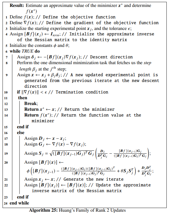
We define a Python function huang() implementing Huang’s family of rank 2 updates . All the other necessary functions and Python codes are left for the reader to fill up according to any example they chose to explore.

def huang(Xj, tol, alpha_1, alpha_2, phi, theta):
    x1 = [Xj[0]]
    x2 = [Xj[1]]
    Bf = np.eye(len(Xj))
    
    while True:
        Grad = Df(Xj)
        delta = -Bf.dot(Grad) # Selection of the direction of the steepest descent
                
        start_point = Xj # Start point for step length selection 
        beta = line_search(f=func, myfprime=Df, xk=start_point, pk=delta, c1=alpha_1, c2=alpha_2)[0] # Selecting the step length
        if beta!=None:
            X = Xj+ beta*delta
        if NORM(Df(X)) < tol:
            x1 += [X[0], ]
            x2 += [X[1], ]
            plt.plot(x1, x2, "rx-", ms=5.5) # Plot the final collected data showing the trajectory of optimization
            plt.show()
            return X, func(X)
        else:
            Dj = X - Xj # See line 17 of the algorithm
            Gj = Df(X) - Grad # See line 18 of the algorithm
            
            den = Dj.dot(Gj)
            num = Bf.dot(Gj)
            
            Sj = au.sqrt(num.dot(Gj))*(Dj/den - num/(num.dot(Gj))) # See line 19 of algorithm
            Bf = phi*(Bf - np.outer(num, num)/(num.dot(Gj)) + theta*np.outer(Sj, Sj)) + np.outer(Dj, Dj)/(Dj.dot(Gj))
            Xj = X # Update to the new iterate
            x1 += [Xj[0], ]
            x2 += [Xj[1], ]

This completes our discussion of Quasi-Newton methods and overall discussion of line-search descent methods.